Day 3 | WISE Workshop — Addis Ababa 2026
2026-02-04
By the end of this session, you will be able to…
Understand why ML and ABM are complementary methodologies
Identify five approaches for integrating ML with agent-based models
Apply ML demand forecasts as ABM agent parameters
Analyze the Beer Game case study and RL-based ordering policies
Connect Days 1-2 forecasting work to Day 4 simulation design
Together: ML provides data-driven predictions that inform mechanistic simulations
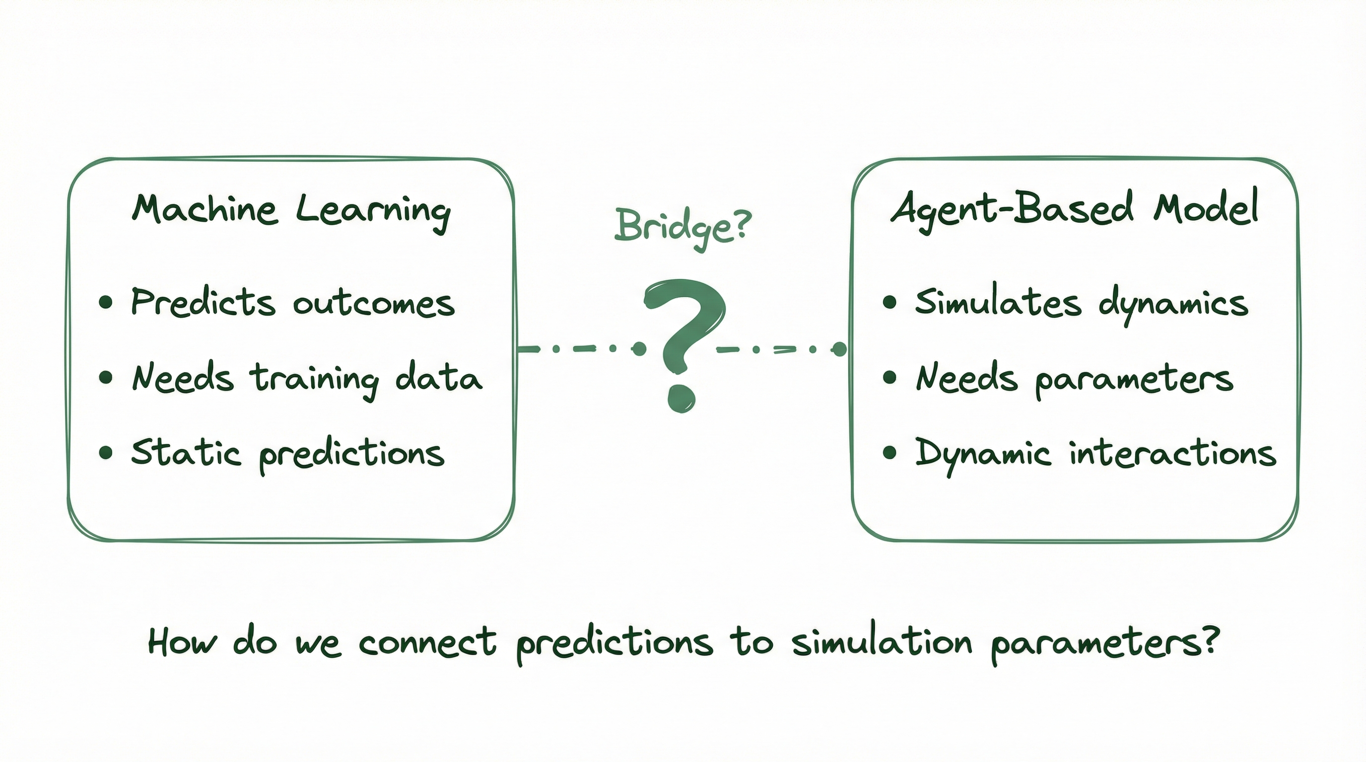
ML and ABM: How do we bridge predictions to simulation parameters?
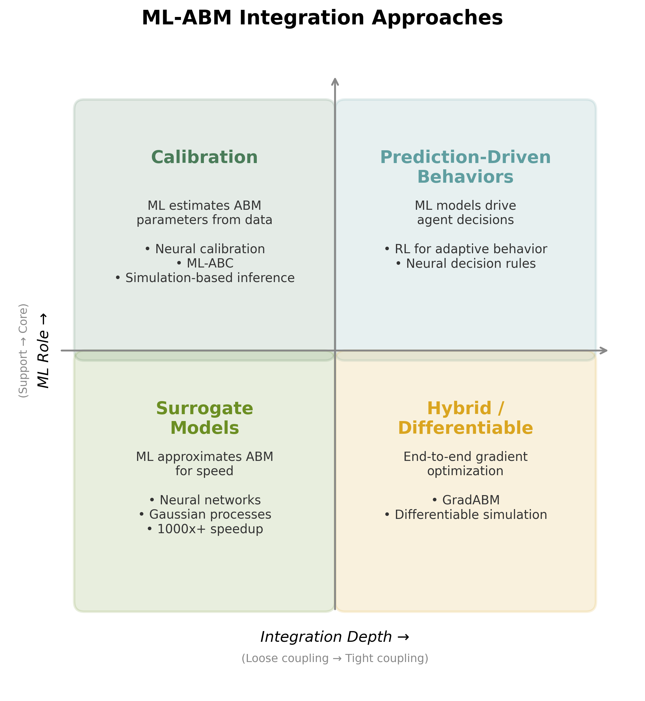
ML-ABM Integration Taxonomy
| Section | Topic | Time |
|---|---|---|
| 1 | Introduction (this section) | 10 min |
| 2 | Integration approaches in depth | 20 min |
| 3 | Case study: Supply chain + RL | 15 min |
| 4 | Reinforcement learning concepts | 10 min |
| 5 | LLM agents (emerging methods) | 10 min |
| 6 | Application to WISE project | 10 min |
| 7 | Health economics applications | 10 min |
| 8 | Wrap-up and discussion | ~5 min |
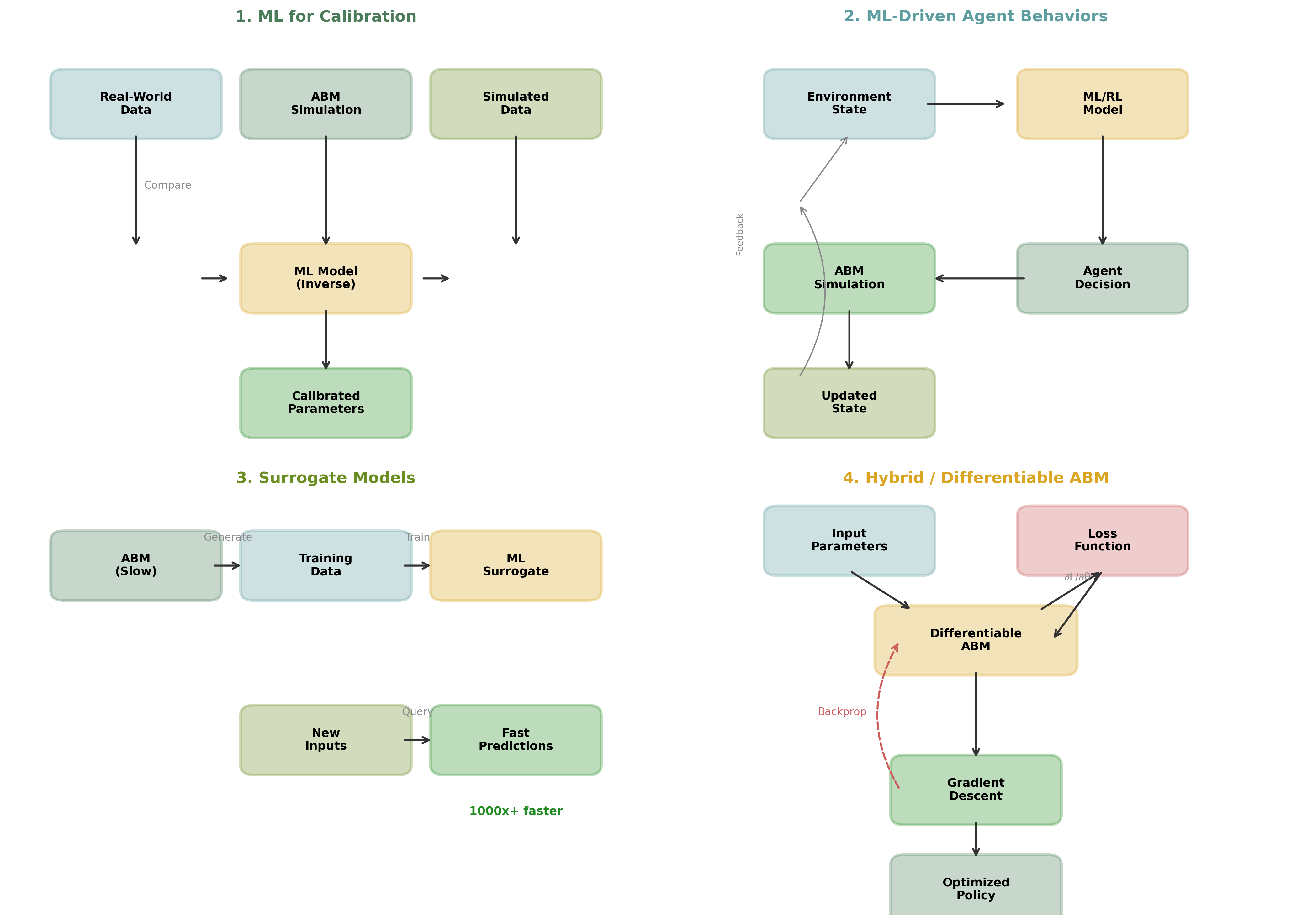
Data flow for each integration approach
Train ML on real-world data → use predictions to parameterize agent decisions
\[\text{Real Data} \xrightarrow{\text{Train ML}} \text{Model} \xrightarrow{\text{Predict}} \text{Agent Parameters}\]
Training:
In ABM:
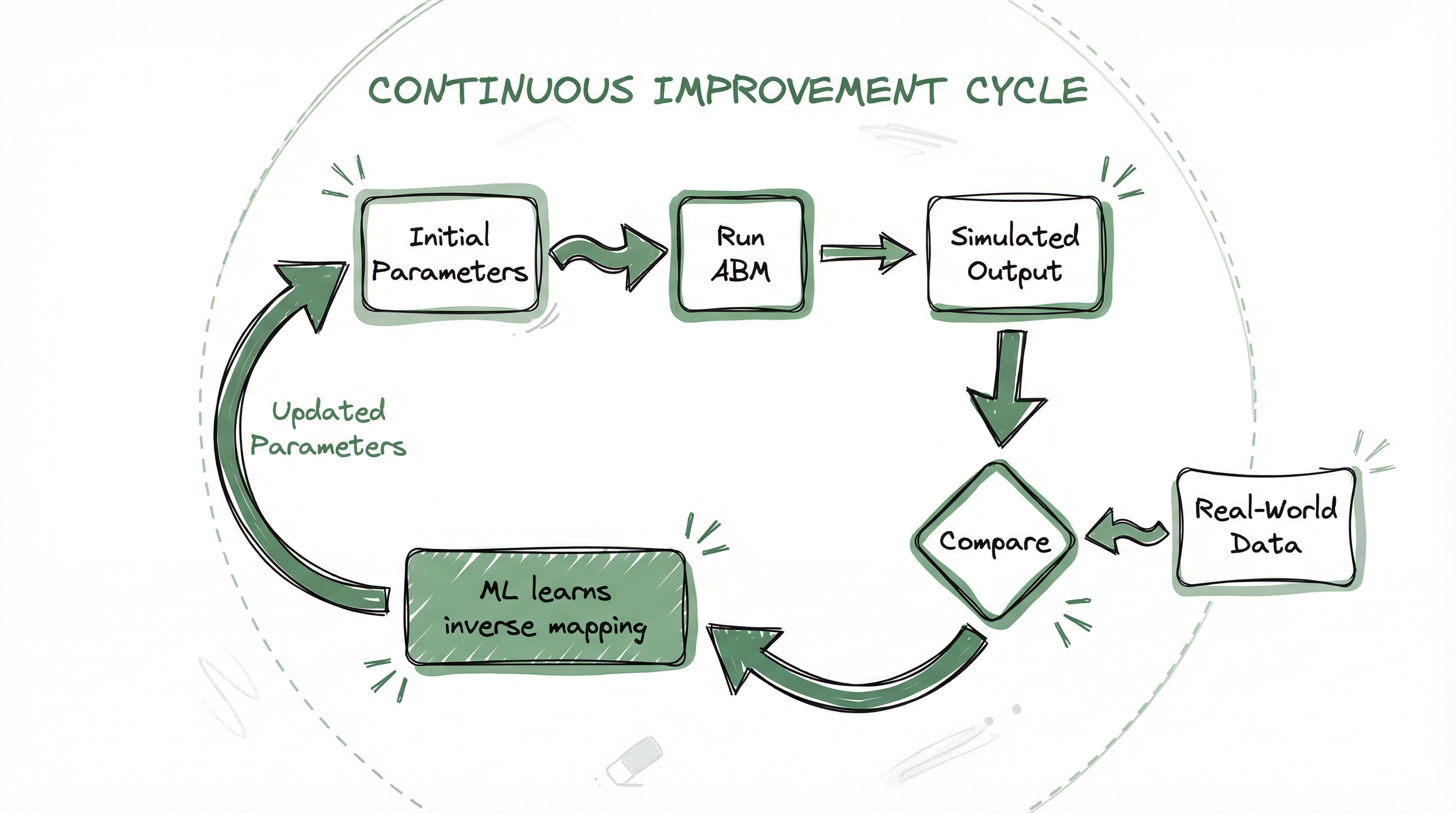
Use ML to learn the inverse mapping:
\[\text{Observed Data} \xrightarrow{\text{ML Model}} \text{ABM Parameters}\]

Neural calibration achieves:
Let ML/RL learn agent decision rules from data or experience:
\[\text{Agent State} \xrightarrow{\text{ML Model}} \text{Agent Decision}\]
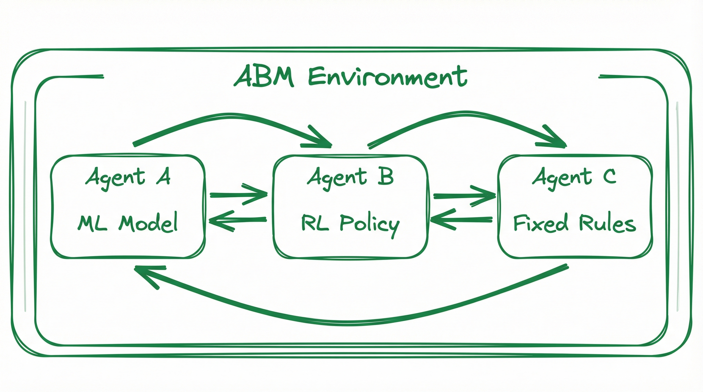
Agents with different decision-making approaches interacting in ABM
Cholera ABM (Zhang et al., 2019):
Train ML to approximate ABM input→output mapping:
\[\text{ABM Inputs} \xrightarrow{\text{Neural Network}} \text{ABM Outputs (Approximate)}\]
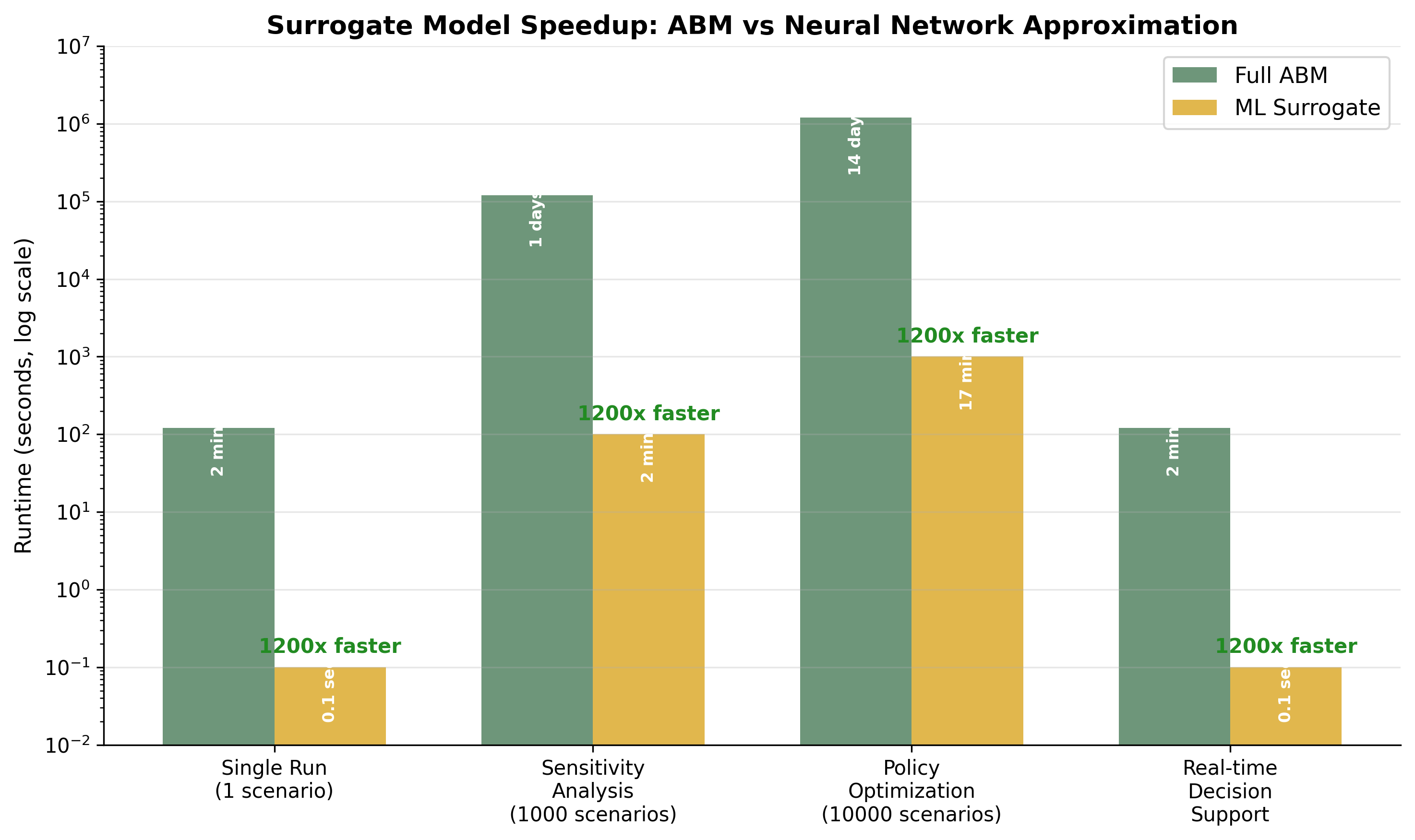
Runtime comparison: Full ABM vs ML Surrogate
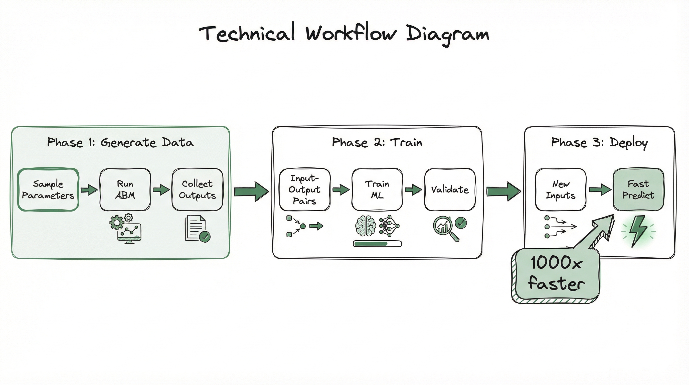
Three-phase surrogate training: Generate data → Train model → Deploy fast predictions
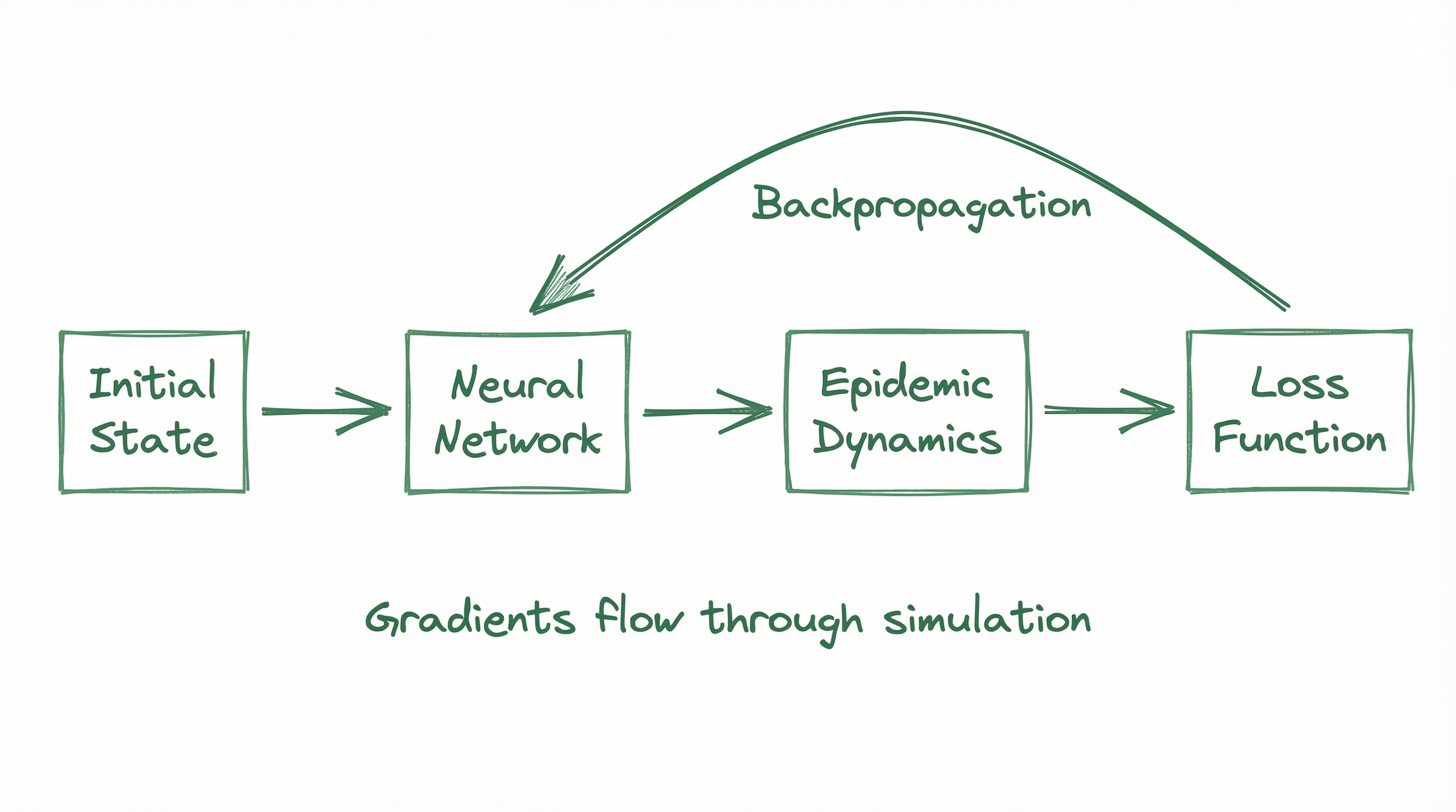
Make ABM differentiable — enable gradient descent:
\[\frac{\partial \text{Loss}}{\partial \text{Parameters}} \xrightarrow{\text{Gradient Descent}} \text{Optimal Policy}\]

| Approach | Use When | Key Benefit |
|---|---|---|
| Calibration | Parameters unknown, have observational data | Automated parameter estimation |
| ML Behaviors | Decision rules complex, have behavioral data | Realistic agent decisions |
| Surrogate | Need many fast runs, computational bottleneck | 1000x+ speedup |
| Hybrid/Diff. | Need end-to-end optimization | Gradient-based policy learning |
| LLM Agents | Cognitive realism, no training budget | Natural reasoning, zero-shot |
Often combine approaches: e.g., ML calibration + surrogate for sensitivity analysis
Manage inventory with only local information
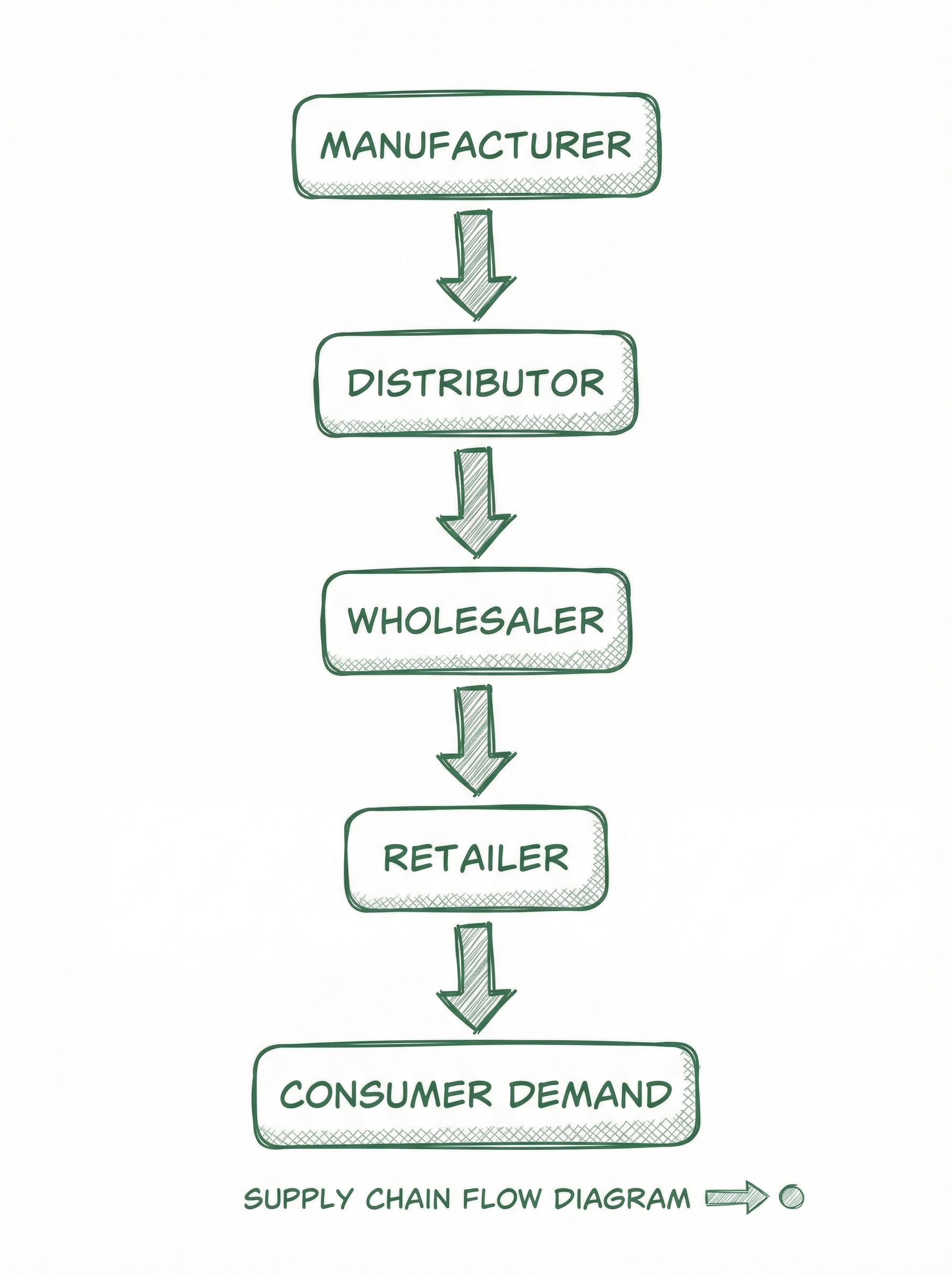
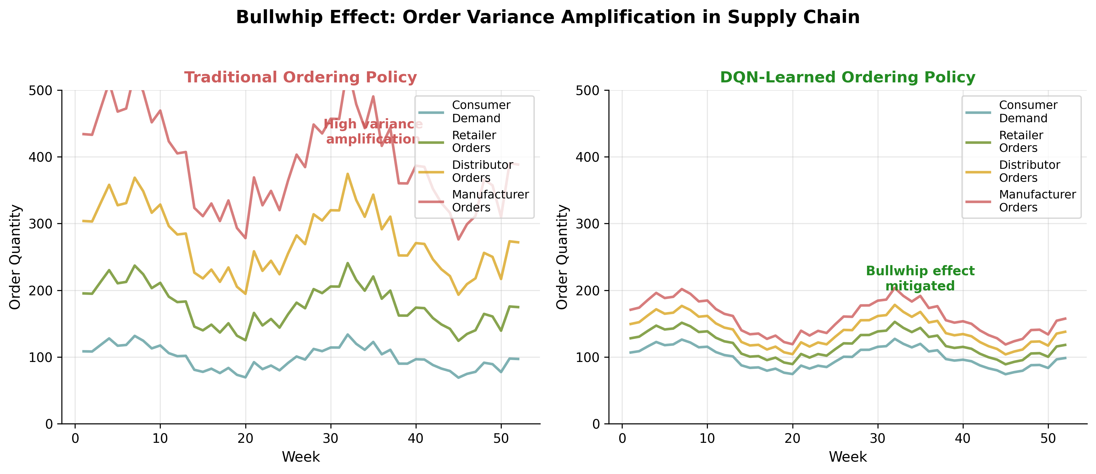
Small demand fluctuations at retail level amplify up the supply chain.
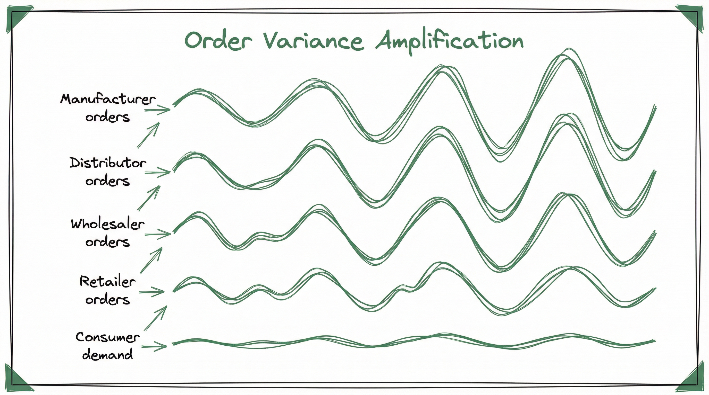
Order variance amplifies upstream in supply chains
Order variance amplification with traditional vs DQN-learned policies
DQN learns to smooth orders even without global information
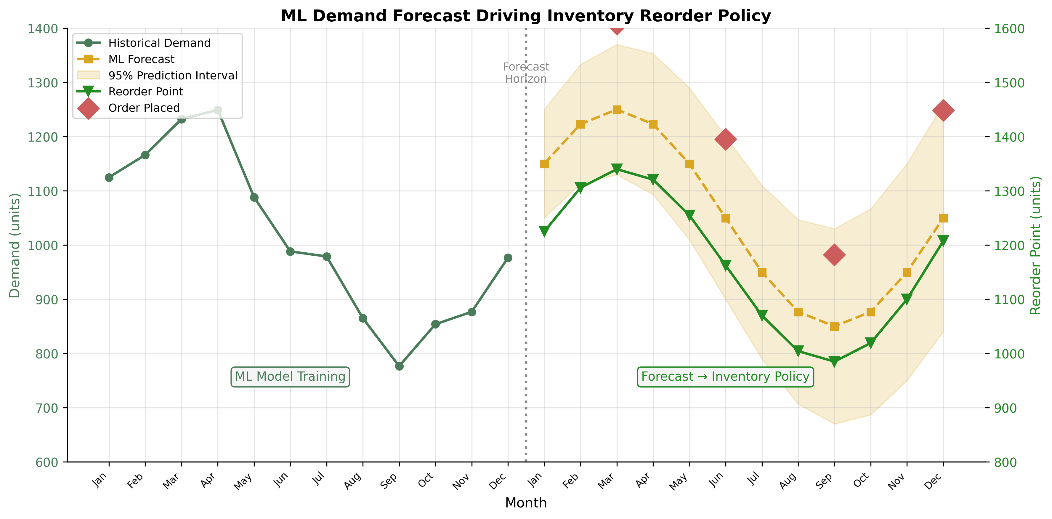
Demand forecast driving inventory reorder decisions
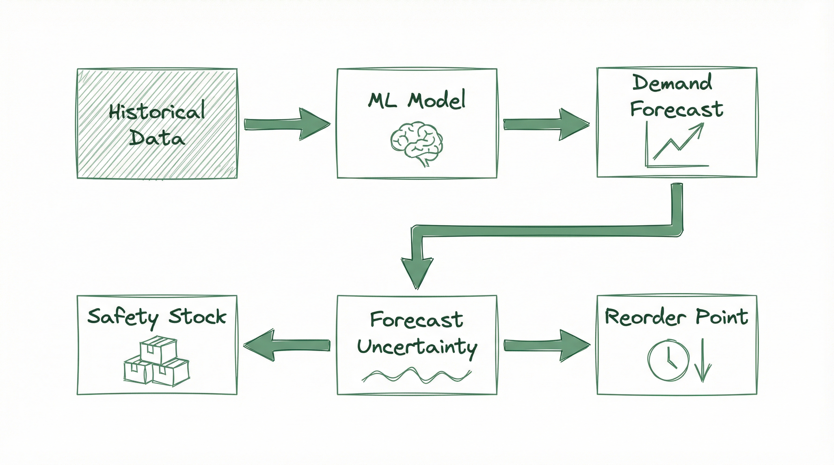
Forecast uncertainty drives safety stock and reorder decisions
Forecast uncertainty (prediction intervals) directly informs safety stock levels
Takeaway: Differentiable ABMs enable rapid policy optimization
ABM serves as the environment in which an RL agent learns
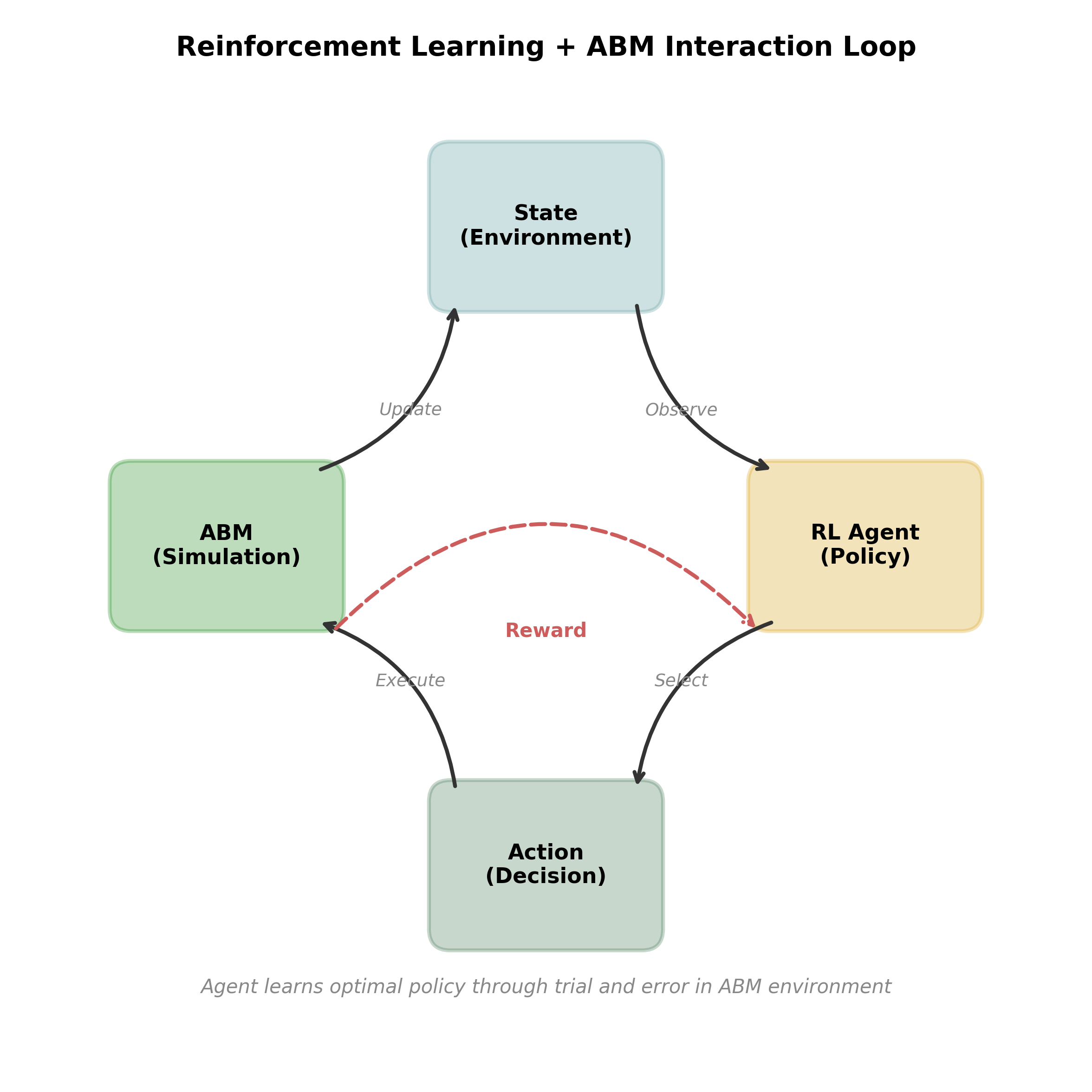
RL-ABM Interaction Loop
| Component | In RL | In Supply Chain ABM |
|---|---|---|
| State | Current observation | Inventory levels, pending orders |
| Action | Decision | Order quantity |
| Reward | Feedback signal | -(holding cost + stockout cost) |
| Policy | Decision rule | Ordering strategy |
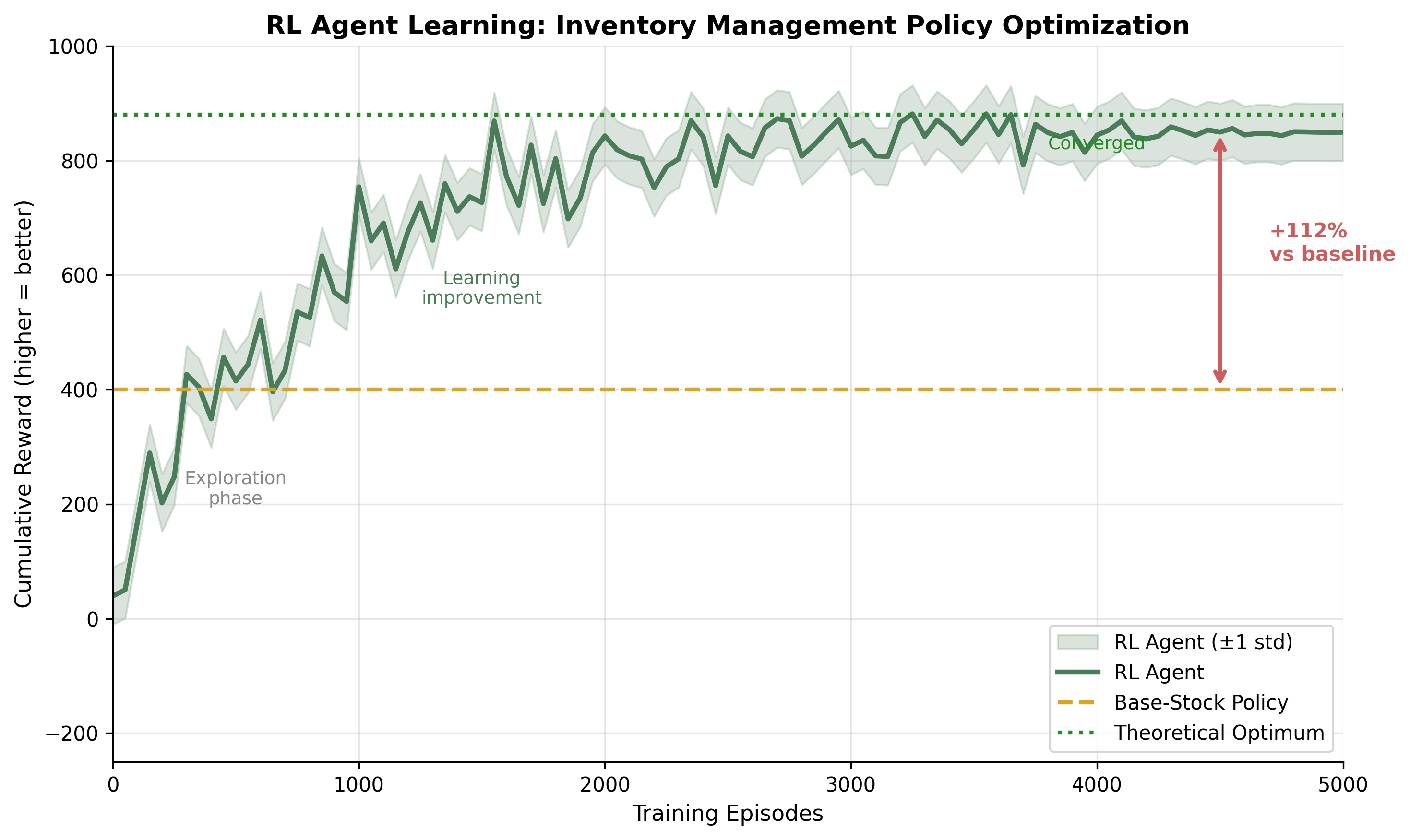
Agent explores actions → observes rewards → updates policy → improves over time
RL agent learning to optimize inventory policy
These are active research areas — resources provided at end for those interested
Inner Loop (Agents):
Outer Loop (Planner):
Supply Chain Analogy:
| AI Economist | Supply Chain |
|---|---|
| Citizens | Facility managers |
| Tax policy | Reorder policies |
| Utility | Minimize costs |
| Govt | Central planner |
AI-designed progressive tax outperformed Saez optimal by +8% on equality-productivity tradeoff

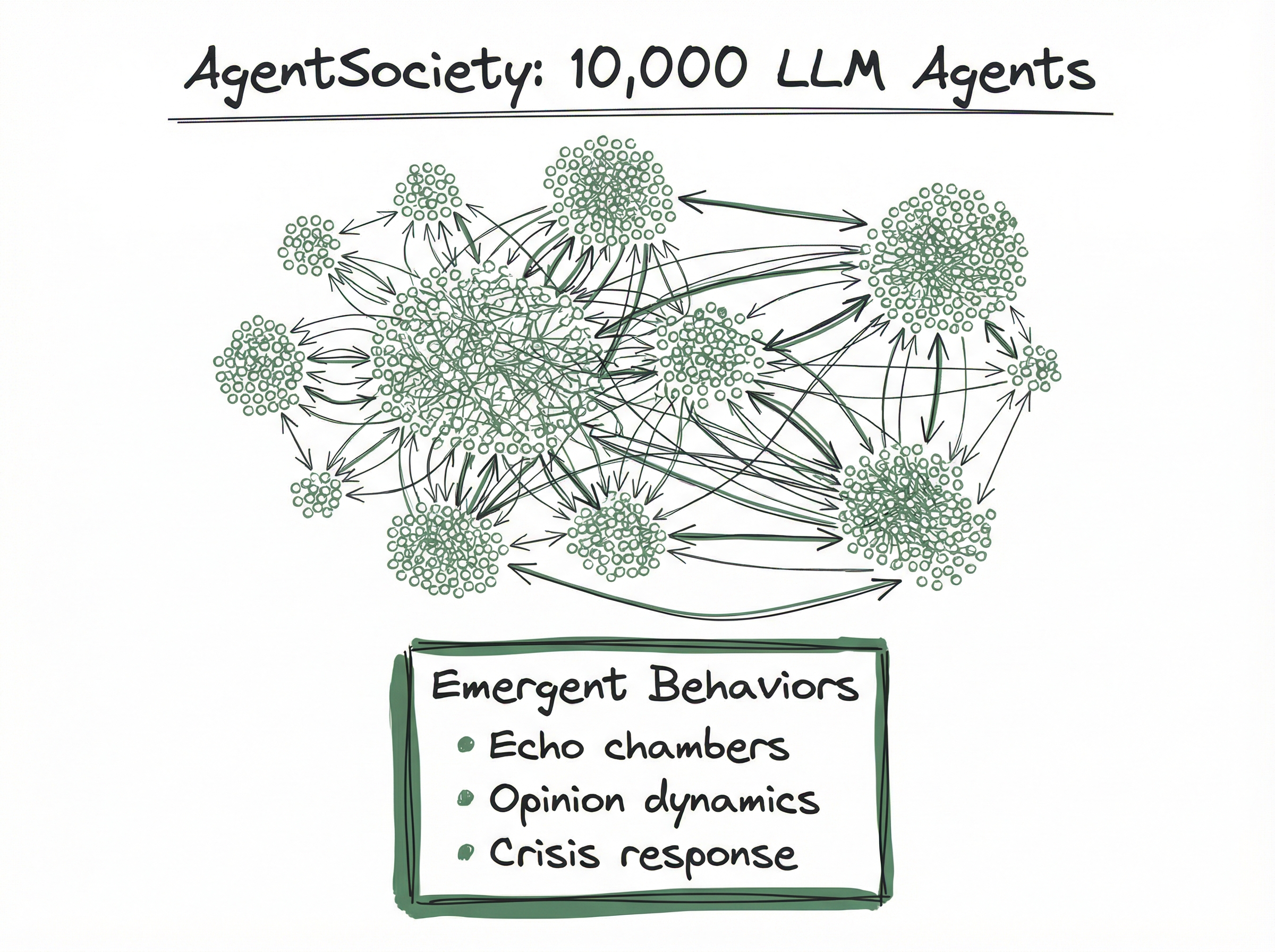
Scale:
Validated Phenomena:

| Dimension | RL Agents | LLM Agents |
|---|---|---|
| Training | Expensive (many simulations) | None (prompt-based) |
| Consistency | High (learned policy) | Variable (stochastic sampling) |
| Reasoning | Implicit (in weights) | Explicit (interpretable) |
| Novel situations | Limited to training distribution | Can handle novel scenarios |
| Cost | Training upfront | Per-inference API calls |
| Behavioral realism | Optimized | Cognitively plausible |
Tradeoff: RL gives optimal behavior; LLM gives realistic behavior
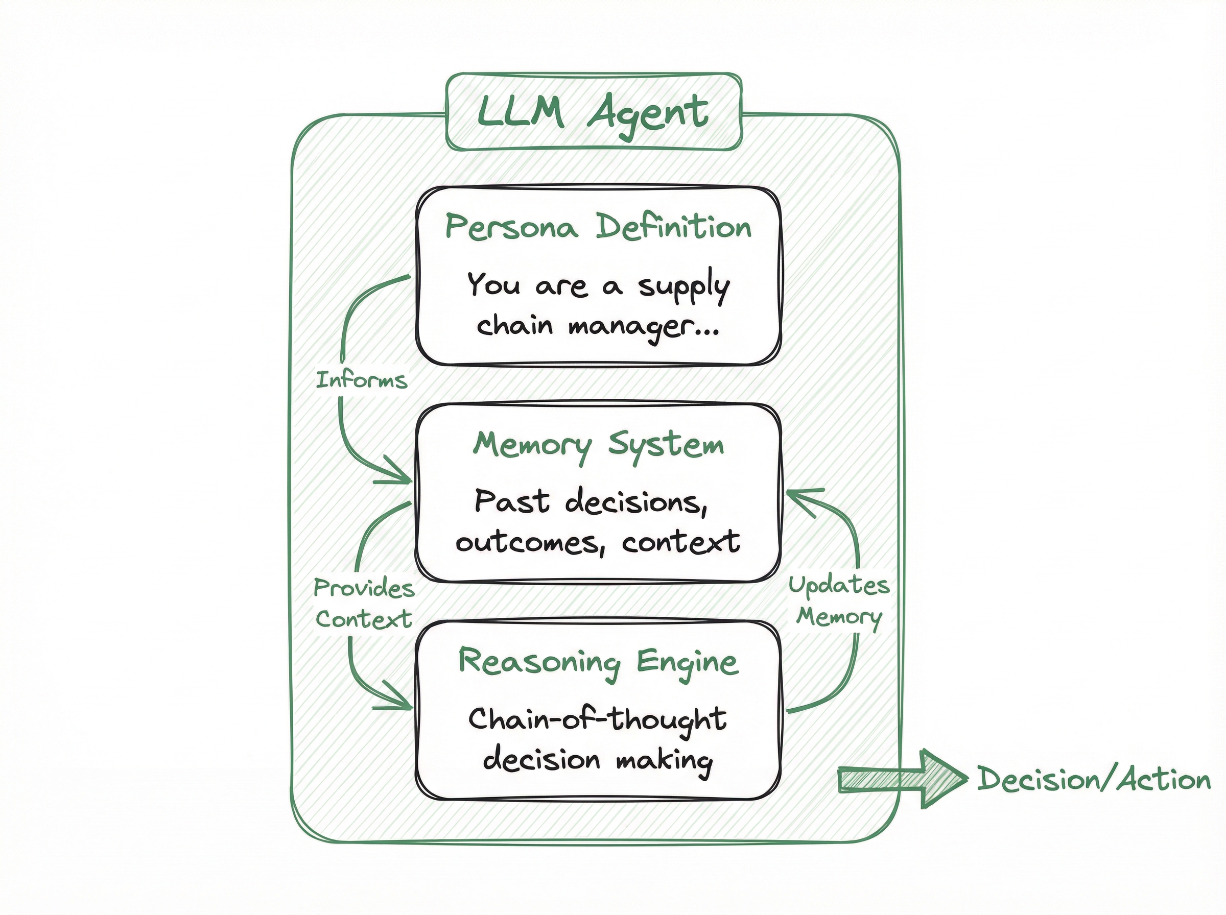
Agent Personas:
Memory Contents:
Why LLM Agents?
Future direction for WISE project?: LLM agents for scenario exploration
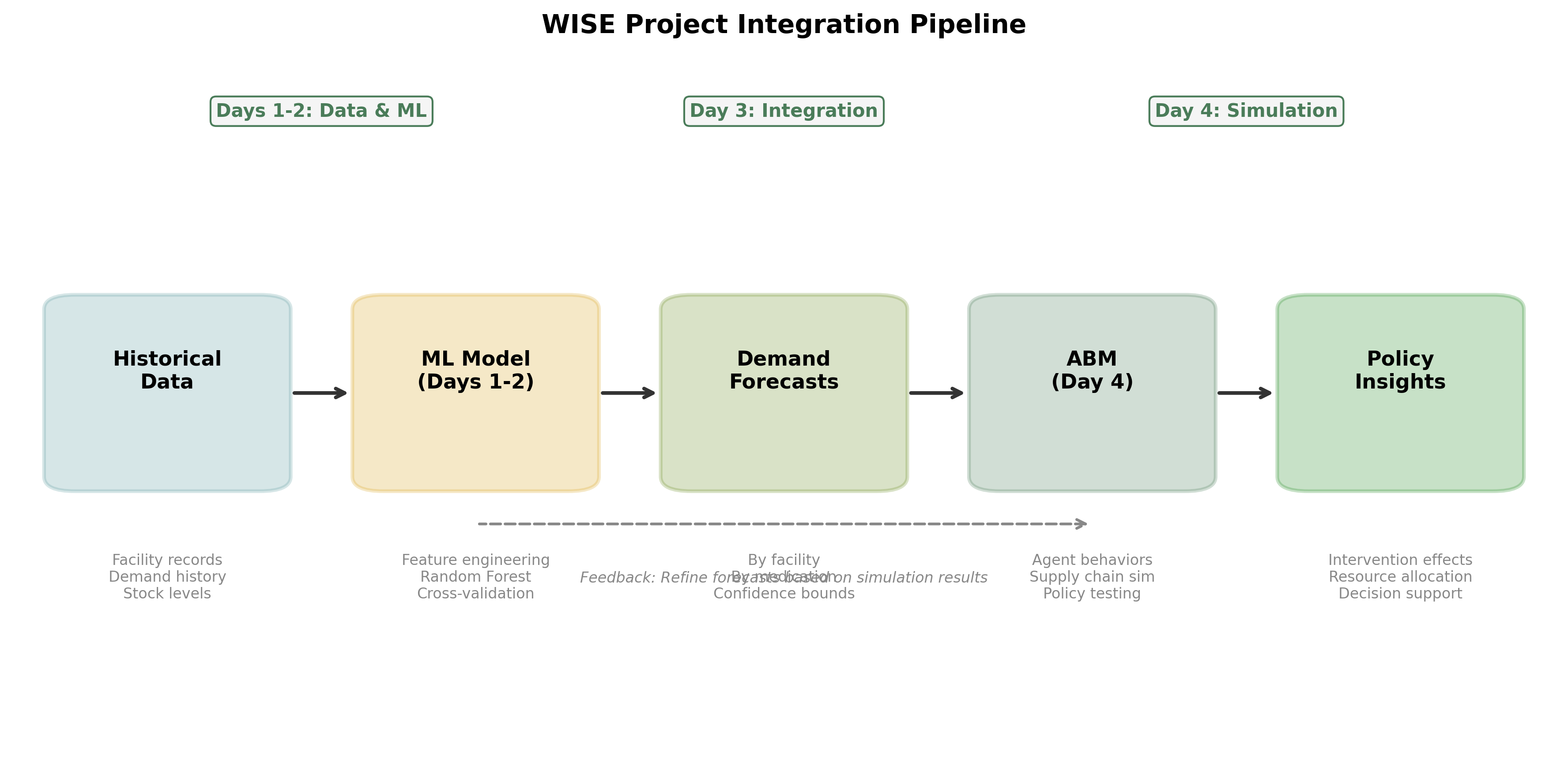
Project workflow from data to policy insights
| Day | Component | Output |
|---|---|---|
| Days 1-2 | ML for demand forecasting | Predictions by facility, medication |
| Day 3 | Integration design (today) | Interface specification |
| Day 4 | ABM simulation | Supply chain model |
| Day 5 | Policy analysis | Intervention recommendations |
Approach 2 (ML-driven behaviors) + elements of Approach 1 (calibration):
# ML Model Output (from Days 1-2)
forecast = {
'facility_id': 'F001',
'medication': 'Amoxicillin 500mg',
'period': '2026-03',
'predicted_demand': 450,
'lower_bound': 380, # 95% CI
'upper_bound': 520
}
# ABM Agent Input (for Day 4)
agent_params = {
'facility_id': 'F001',
'reorder_point': 520, # upper_bound for safety
'order_quantity': 450, # predicted demand
'lead_time': 14, # days
'review_period': 30 # days
}You built ML models to predict antibiotic demand by facility
We’ll build a supply chain ABM where agents make ordering decisions
| Your Situation | Recommended Approach |
|---|---|
| Have behavioral data, want realistic agents | ML as Parameters (Approach 1) |
| Unknown parameters, need calibration | ML Calibration (Approach 2) |
| Complex decisions, adaptive behavior needed | ML/RL Behaviors (Approach 3) |
| Need fast scenario sweeps | Surrogate Models (Approach 4) |
| Policy optimization, gradient-based | Hybrid/Differentiable (Approach 5) |
| Cognitive realism, no training budget | LLM Agents (emerging) |
WISE Project: Approach 1 (ML forecasts → ordering parameters) + potential Surrogate for sensitivity
Problem: Evaluate shared savings contracts
Integration: - ML predicts patient risk - ABM simulates care decisions - Surrogate enables contract optimization
Outcome: Optimal risk corridor design
Problem: Will clinicians use AI tools?
Integration: - LLM agents simulate physician reasoning - ABM captures workflow constraints - RL learns optimal nudge policies
Outcome: Adoption pathway recommendations
Problem: Vaccine prioritization strategy
Integration: - ML calibrates transmission from data - Differentiable ABM enables gradient-based optimization - Fast counterfactual analysis
Outcome: Age-stratified priority schedules
Phase 1: Calibrate
Phase 2: Surrogate
Phase 3: Sweep
Phase 4: Validate
This workflow combines multiple integration approaches for robust policy analysis
ML forecasts → ABM parameters → Policy simulation
| Topic | Reference |
|---|---|
| Integration review | Zhang et al. (2021). IEEE TNNLS |
| Differentiable ABM | Chopra et al. (2023). AAMAS |
| Surrogate modeling | Angione et al. (2022). PLOS ONE |
| Neural calibration | Gaskin et al. (2023). PNAS |
| Beer Game DQN | Oroojlooyjadid et al. (2021). M&SOM |
| LLM agent society | Piao et al. (2025). arXiv |
Supply Chain Simulation Foundations
Full ABM Development
For the WISE project supply chain, which integration approach seems most promising? Why?
What data would we need to train an RL agent for inventory management?
How might we validate that our ML → ABM integration produces realistic results?
WISE Workshop | Data Sciences for Modeling & HTA