Tree-based Methods

Day 2 Afternoon | WISE Workshop — Addis Ababa 2026

Sean Sylvia, Ph.D.

2026-02-03

Unit 2: Basic ML Crash Course

  1. Introduction to ML

  2. Lasso and friends (Linear High-dimensional Regression)

  3. Tree-based methods (Nonlinear)

Review

Basic ML Setup

  1. Flexible functional forms

  2. Limit expressiveness via regularization

  3. Learn how much to regularize tuning

  • What do the features imply about properties of \(\hat{f}\) ?
  • How can we use \(\hat{f}\) in applied data analyses?

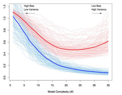
The Approximation-Overfit Tradeoff

The Fundamental Challenge

As model complexity increases, we face two competing forces:

  1. Approximation error decreases as we better capture the true underlying function
  2. Estimation error increases as we begin to fit noise in our training data

This creates the bias-variance tradeoff that defines machine learning:

  • Simple models: High bias, low variance
  • Complex models: Low bias, high variance

Bias-variance tradeoff visualization. The blue curve represents test error, while the red curve shows training error. The gap widens as model complexity increases, indicating overfitting.

Supervised Learning

For supervised learners, we need three things:

  1. Function Class
  2. A regularizer
  3. Optimization algorithms to guide us

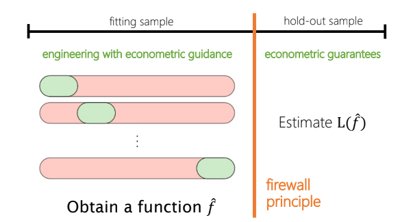
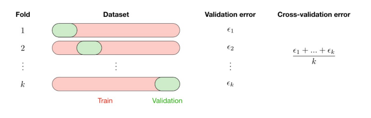
Choosing a regularization parameter using k-fold Cross-validation

Full ML Exercise

The Regularization Spectrum: How We Control Complexity

Every model class has its own unique form of regularization that controls the bias-variance tradeoff. Understanding this spectrum reveals the fundamental unity behind seemingly diverse machine learning approaches.

Function Class Regularization Parameters
Linear LASSO, ridge, elastic net
Decision/regression trees Depth, leaves, leaf size, info gain
Random forest Trees, variables per tree, sample sizes, complexity
Nearest neighbors Number of neighbors
Kernel regression Bandwidth
Splines Number of knots, order
Neural nets Layers, sizes, connectivity, drop-out, early stopping

Cross-cutting insight: While the specific mechanisms differ, regularization always involves restricting a model’s capacity to memorize training data, instead encouraging it to generalize underlying patterns. Tree-based methods share this fundamental principle with linear models, but implement it through structural constraints rather than coefficient penalties.

Lasso Regression: Constrained Minimization to Regularize

Objective: Minimize the sum of squared errors while keeping coefficients small

Constrained Form

\[ \begin{align} \min_{\beta} &\sum_{i=1}^{n} \left(y_i - \beta_0 - \sum_{j=1}^{p} \beta_j x_{ij}\right)^2\\ \text{subject to } &\sum_{j=1}^{p} |\beta_j| \leq t \end{align} \]

  • \(t \geq 0\) is the constraint parameter
  • Smaller \(t\) means more regularization
  • \(t = 0\) forces all \(\beta_j = 0\)

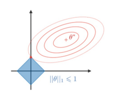
Contours of RSS function and lasso constraint region (diamond). Solution occurs at corners, forcing coefficients to zero.

Lasso: Lagrangian Form

\[ \min_{\beta} \sum_{i=1}^{n} \left(y_i - \beta_0 - \sum_{j=1}^{p} \beta_j x_{ij}\right)^2 + \lambda \sum_{j=1}^{p} |\beta_j| \]

  • \(\lambda \geq 0\) is the penalty parameter
  • \(\lambda\) and \(t\) have an inverse relationship
  • As \(\lambda \rightarrow \infty\), all \(\beta_j \rightarrow 0\)

Geometric Interpretation

  • The constraint region: \(\sum_{j=1}^{p} |\beta_j| \leq t\) forms a diamond (L1 norm)
  • Unlike ridge regression’s circular constraint (L2 norm)
  • Key insight: The corners of the diamond often intersect with axes
  • This means some coefficients become exactly zero

Contours of RSS function and lasso constraint region (diamond). Solution occurs at corners, forcing coefficients to zero.

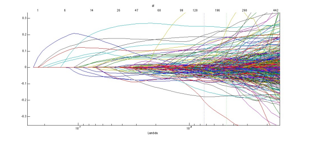
Lasso Lambda and coefficient paths (relaxing constraint)

Each line is a coefficient. Lambda is “relaxed” moving from left to right

Why Lasso Performs Variable Selection

The L1 penalty’s diamond shape makes it likely for solutions to occur at corners where some \(\beta_j = 0\)

  • Solution occurs where RSS contours touch constraint region
  • Corners of diamond intersect with coordinate axes
  • When solution is at a corner, some coefficients equal zero
  • Result: Automatic variable selection

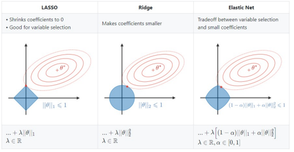
Comparison of lasso (diamond) vs. ridge (circle) vs. elastic net (fat diamond thingy) constraint regions.

The Lasso Selection Problem

Challenge: Different regularization paths can lead to different selected variables

OLS:
Health = β₀ + β₁·Age + β₂·Income + β₃·Education + β₄·SES + … + βₙ·X_n + ε

Lasso (1):
Health = β₀ + β₁·Age + β₂·Income + β₃·Education + … + βₙ·X_n + ε

Lasso (2):
Health = β₀ + β₁·Age + + β₄·SES + … + βₙ·X_n + ε

Lasso Selection Problem

Key implications:

  • Variable selection depends heavily on choice of λ
  • Highly correlated predictors compete for selection
  • Different random seeds in cross-validation → different final models
  • Selection can be unstable with small changes in data

Lasso Selection Instability

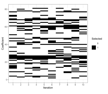
Lasso variable selection often exhibits instability across different runs, even on the same dataset:

  • Small changes in data can lead to completely different sets of selected variables
  • Highly correlated predictors compete for selection
  • Cross-validation randomness affects final model composition
  • Bootstrapping or repeated CV shows selection frequencies

Implications for practice: - Single Lasso runs may miss important variables - Ensemble approaches can provide more stable selection - Variable selection consistency is not guaranteed

Variable selection across 10 iterations of Lasso on the same dataset. Black indicates selected; white indicates excluded. Notice the inconsistent pattern of selection.

Tree-Based Methods: Overview

  • Previously: linear models, regularization (ridge, lasso, elastic net)
  • Now: flexible, non-parametric approaches for prediction and classification

Key Question:

How can we model non-linear relationships without assuming functional form?

Decision trees and (mostly) their extensions…

Tree-based methods include random forests, bagged trees, boosted trees, which combine many decision trees in different ways (called an ensemble)..

Why Tree-Based Methods?

  • Powerful non-parametric approaches that:
    • Make no assumptions about functional form
    • Automatically model interactions between predictors
    • Handle different types of predictors (continuous, categorical)
    • Are highly interpretable (single trees)
    • Can achieve excellent predictive performance (ensembles)

Perfect for health services research, where relationships are often complex and non-linear!

Decision Trees: Intuition

  • Trees reflect human decision-making processes
  • We navigate a series of yes/no questions
  • Arrive at a prediction based on answers to those questions

Trees segment predictor space into regions, then:

  • For regression: Predict mean outcome value in that region
  • For classification: Predict most common class in that region

The beauty is in the simplicity: - No formula needed - Can capture complex relationships without parametric assumptions

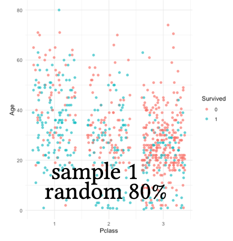
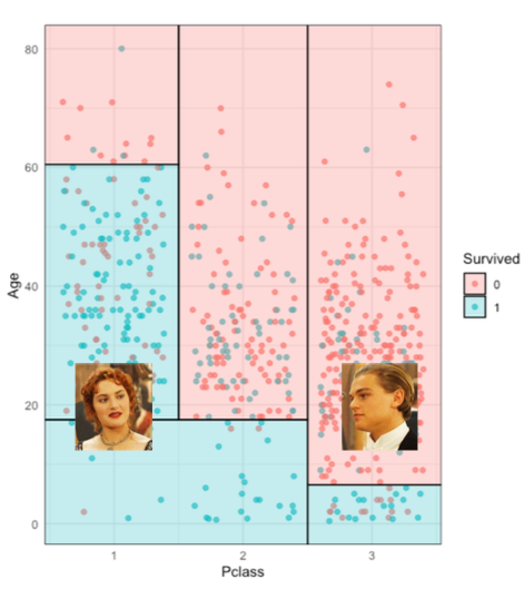
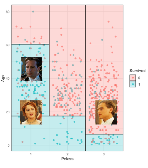
Example: Surviving the Titanic

Example: Surviving the Titanic

Age, Class and Survival

Age, Class and Survival

Age, Class and Survival

Age, Class and Survival

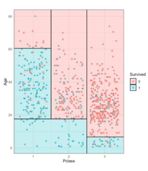
Age, Class and Survival: Tree

flowchart TD
    A[Age > 60?] --> |Yes| B[Did not survive]
    A --> |No| C[Pclass = 1?]
    C --> |Yes| D[Survived]
    C --> |No| E[Pclass = 2?]
    E --> |Yes| F[Age > 20?]
    F --> |Yes| G[Did not survive]
    F --> |No| H[Did not survive]
    E --> |No| I[Age < 10?]
    I --> |Yes| J[Survived]
    I --> |No| K[Did not survive]

    %% Styling
    classDef survived fill:#a8d5e5,stroke:#333,stroke-width:1px;
    classDef notSurvived fill:#f8cecc,stroke:#333,stroke-width:1px;

    class D,J survived;
    class B,G,H,K notSurvived;

How to Grow a Tree?

The general approach:

  1. Split: Choose a predictor and value to split data
  2. Recurse: Apply the same process to resulting regions
  3. Prune: Simplify the tree to prevent overfitting

The key challenge: Finding the optimal splits

Growing a Regression Tree

Goal: Partition predictor space into non-overlapping regions \(R_1, R_2, ..., R_J\) to minimize:

\[RSS = \sum_{j=1}^{J} \sum_{i \in R_j} (y_i - \hat{y}_{R_j})^2\]

Where \(\hat{y}_{R_j}\) is the mean response for observations in region \(R_j\)

Recursive Binary Splitting

  1. Consider all predictors \(X_j\) and all possible cut points \(s\)
  2. For each combination, split predictor space into two regions: \[R_1(j,s) = \{X|X_j < s\} \text{ and } R_2(j,s) = \{X|X_j \geq s\}\]
  3. Choose split that minimizes: \[\sum_{i \in R_1(j,s)} (y_i - \hat{y}_{R_1})^2 + \sum_{i \in R_2(j,s)} (y_i - \hat{y}_{R_2})^2\]
  4. Repeat recursively on each resulting region

Classification Trees

  • Used when predicting categorical outcomes
  • Same recursive splitting approach, but different splitting criteria
  • Instead of RSS, we use measures of node purity

Common impurity measures: - Classification Error Rate: \(1 - \max_k(p_{mk})\) - Gini Index: \(\sum_{k=1}^K p_{mk}(1-p_{mk})\) - Entropy: \(-\sum_{k=1}^K p_{mk}\log(p_{mk})\)

Where \(p_{mk}\) is the proportion of observations in node \(m\) that belong to class \(k\)

Prediction with Trees

Once the tree is built:

  • Regression: Predict the mean response value in the leaf node
  • Classification: Predict the most common class in the leaf node

Trees can also provide probability estimates (proportions of classes in each node)

Advantages of Trees

  • Interpretability: Easy to explain and visualize
  • No preprocessing needed: No normalization or dummy variables required
  • Handle mixed data types: Both numerical and categorical predictors
  • Automatically model interactions
  • No distributional assumptions
  • Handle missing data (with appropriate implementation)

Disadvantages of Trees

  • High variance: Small changes in data can result in very different trees
  • Can overfit: Tend to learn noise in the data if not constrained
  • Greedy algorithm: May not find global optimum
  • Limited predictive accuracy (for single trees)
  • Biased toward predictors with many possible splits

The Overfitting Challenge

  • Deep trees fit training data perfectly but generalize poorly
  • Need a way to find right-sized trees

Tree Pruning

  • Idea: Grow a large tree, then prune it back to prevent overfitting
  • Approach: Cost-complexity pruning with a penalty for tree complexity

Find subtree \(T \subset T_0\) that minimizes:

\[\sum_{m=1}^{|T|} \sum_{i:x_i \in R_m} (y_i - \hat{y}_{R_m})^2 + \alpha|T|\]

where \(|T|\) is the number of terminal nodes and \(\alpha\) is the complexity parameter

Cross-Validation for Optimal Tree Size

  1. Grow a large tree \(T_0\)
  2. For range of \(\alpha\) values, find best subtree \(T_\alpha\)
  3. Use K-fold cross-validation to select optimal \(\alpha\)
  4. Return the subtree \(T_\alpha\) that corresponds to the optimal \(\alpha\)

Remember: We’re using the same cross-validation framework we learned with lasso!

The Fundamental Problem of Trees

Single trees have: - High interpretability - Limited predictive performance

Can we keep the flexibility of trees while improving predictive performance?

Ensemble Methods to the Rescue!

The core idea: Combine many trees to reduce variance and improve predictions

Key ensemble approaches:

  1. Bagging: Bootstrap aggregation of trees
  2. Random Forests: Bagging with random feature selection
  3. Boosting: Sequential tree building to correct errors

Bagging Trees

Bagging Trees

Bagging (Bootstrap Aggregation)

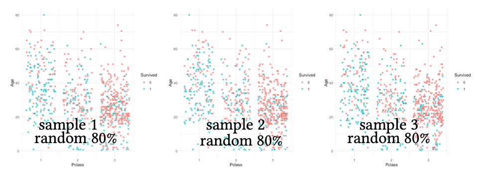
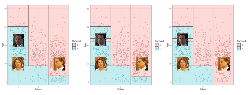
  1. Create \(B\) bootstrap samples from training data
  2. Fit a deep, unpruned tree to each bootstrap sample
  3. Average predictions across all trees (for regression)
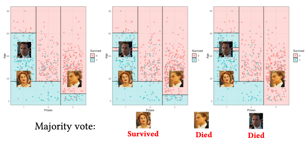
  4. Take majority vote (for classification)

Key insight: Averaging many high-variance, low-bias estimators gives a lower-variance, low-bias ensemble

Ensemble Prediction

By averaging over many low bias but high variance models, we reduce the overall variance ⇒ more accurate model.

  • the average of all \(B\) predictions for regression trees: \(\hat{y}_{bag}(X) = \frac{1}{B} \sum_{i=1}^{B} \hat{y}^i(X)\)

  • the majority vote by all \(B\) predictions for classification trees: \(\hat{y}_{bag}(X) = \underset{k}{\arg\max} \sum_{i=1}^{B} I\{\hat{y}^i(X) = k\}\)
flowchart TB
    Forecast["Forecast for any new X"] --> DT1["DT 1<br>sample 1<br>random S%"]
    Forecast --> DT2["DT 2<br>sample 2<br>random S%"]
    Forecast --> dots1["..."]
    Forecast --> dots2["..."]
    Forecast --> dots3["..."]
    Forecast --> DTB["DT B<br>sample B<br>random S%"]

Majority Vote

Out-of-Bag Error Estimation

  • Each bootstrap sample only uses ~2/3 of observations
  • Remaining ~1/3 (“out-of-bag” or OOB) can be used as validation data
  • For each observation, average predictions from trees that didn’t use it in training
  • Provides honest error estimate without separate validation set

Random Forests: Decorrelating Trees

Random forests address a weakness of bagging:

  • In bagging, trees can be highly correlated if strong predictors dominate splits

Random forests solution:

  • At each split, consider only a random subset of \(m\) predictors

  • Typically \(m \approx \sqrt{p}\) for classification, \(m \approx p/3\) for regression

  • For example, with sample of 100 predictors, sample 10 in each split for class.

  • Decorrelates trees, further reducing variance

Random Forest are Particularly useful when there is one strong predictor or a set of predictors that are highly correlated with each other. (Why?)

Boosting: Sequential Learning

Unlike bagging/random forests (parallel tree building), boosting:

  • Fits trees sequentially

  • Each tree focuses on errors of previous trees

  • Combines many “weak learners” into a strong ensemble

Key insight: Rather than averaging many independent predictions, we build an additive model of trees

Gradient Boosting Algorithm

For regression (simplified):

  1. Initialize \(\hat{f}(x) = 0\)

  2. For \(b = 1\) to \(B\):

    • Compute residuals \(r_i = y_i - \hat{f}(x_i)\)

    • Fit a small tree to the residuals, get predictions \(\hat{h}_b(x)\)

    • Update model: \(\hat{f}(x) = \hat{f}(x) + \lambda \hat{h}_b(x)\)

    • Where \(\lambda\) is the learning rate (shrinkage parameter)

Boosting Tuning Parameters

Three key parameters control the model:

  1. Number of trees \(B\): More trees can improve performance but may lead to overfitting

  2. Tree depth \(d\): Controls complexity of individual trees (often shallow, 1-6 nodes)

  3. Learning rate \(\lambda\): How quickly model adapts to errors (smaller values need more trees)

As with other regularization approaches, cross-validation helps select optimal parameters

Gradient Boosting vs. Random Forests

Random Forests

  • Trees built independently

  • Try to average out errors

  • Less prone to overfitting

  • Easier to tune

Gradient Boosting - Trees built sequentially

  • Try to correct previous errors

  • More prone to overfitting

  • Often higher accuracy, if tuned properly

XGBoost: State-of-the-Art Boosting

  • eXtreme Gradient Boosting (XGBoost) is a highly optimized boosting implementation

  • Regularization term in objective function

  • Efficient handling of sparse data

  • Parallel processing

  • Often wins machine learning competitions

XGBoost Objective:

\[\text{Obj} = \sum_{i=1}^n l(y_i, \hat{y}_i) + \sum_{k=1}^K \Omega(f_k)\]

Where \(\Omega(f) = \gamma T + \frac{1}{2}\lambda ||\omega||^2\) penalizes complex trees

Applications in Health Services Research

  • Predicting hospital readmissions: Capturing complex interactions between comorbidities
  • Identifying high-risk patients: Finding non-linear patterns in health indicators
  • Claims data analysis: Handling mixed data types from administrative datasets
  • Medical imaging: Feature extraction and classification
  • Treatment effect heterogeneity: Identifying subgroups with different responses to interventions

Tuning Tree-Based Methods

  • Single trees: Prune using cross-validation to select complexity parameter
  • Bagging: Typically only need to set number of trees (usually 100-500)
  • Random Forests: Number of trees and mtry (predictors per split)
  • Boosting: Number of trees, learning rate, tree depth

Remember: Cross-validation is essential for all these models!

Key Takeaways

  1. Tree-based methods offer flexible, non-parametric modeling
  2. Single trees prioritize interpretability
  3. Ensemble methods dramatically improve predictive performance
  4. Random Forests: Easy to tune, robust performance
  5. Boosting: Often highest accuracy, but requires careful tuning
  6. Tree ensembles provide variable importance and partial dependence for interpretation

Next Steps

  • Lab exercise: Implementing tree-based methods in R
  • Readings: Chapter 8 in “Introduction to Statistical Learning”
  • Coming up: Causal trees and forests - using tree-based methods for causal inference!

Prediction vs. Estimation

  • Prediction: Out-of-sample loss minimization \(\rightarrow\) \(\hat{y}\)
  • Estimation: Coefficient inference \(\rightarrow\) \(\hat{\beta}\)
  • In high dimensions:
    • Good predictions possible even if \(\hat{\beta}\) is unstable/biased
    • Multiple functions can predict similarly; distinguishing is hard
    • Regularization & tuning help prediction but complicate estimation

Prediction \((\hat{y})\)

  • ML prediction aims for a good fit of \(\hat{y}\) to \(y\) on the same distribution
  • Not necessarily about policy counterfactuals or structural knowledge
  • Counterfactual analysis requires causal modeling

Estimation \((\hat{\beta})\)

  • Some ML approaches estimate \(f(x) \approx \mathbb{E}[y \mid x]\)
  • Achieving minimal loss does not guarantee consistent \(\hat{\beta}\) for inference
  • Consistency depends on the distribution of \(x\)
  • Structural parameters require more than just good fit

Key Takeaways for Applied Work

  • ML excels at predicting \(\hat{y}\)
  • Hold-out or cross-validation validate prediction quality
  • Typically no consistency for \(\hat{\beta}\)
  • Limited causal interpretation or counterfactual extrapolation
  • Inference can be tricky; bootstrap may fail in high dimensions

Application Areas for a \(\hat{y}\) Tool

  1. Data pre-processing
  2. \(\hat{y}\) tasks (prediction policy problems)
  3. \(\hat{y}\) in service of \(\hat{\beta}\)